Tuesday, February 24, 2015

Electron Cont'd (9)

We're now ready to discuss some results from our JSBSim flight dynamics simulation. In this post, we'll talk mainly about how to survive maximum aerodynamic pressure, or max q.
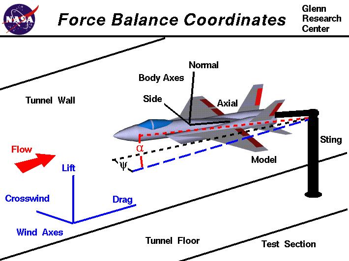
Let's begin by defining the coordinate systems used for our rocket, as well as major forces and velocities involved.


The engines produce a forward thrust that pushes the rocket along the direction of velocity V. Most liquid rocket engines require a little bit of time to develop enough thrust to be able to lift the combined mass of the rocket plus fuel and oxidizer off the ground. During this short period, a hold down mechanism is typically used to keep the rocket stable on the pad. While the rocket is flying within the atmosphere, a drag force due to air resistance (wind) directly opposes the rocket's thrust.

If the rocket's velocity vector is not aligned with the actual pitch angle with the horizon, the resulting angular difference is called the angle of attack alpha. A large alpha may result in a strong perpendicular lifting force due to aerodynamic lift. This is usually bad, because for a long object such as a rocket, excessive perpendicular forces could cause the rocket to bend and result in structural failure. Thus many rockets aim to fly a zero angle of attack and throttle back during flight through max q. This reduces bending forces to a manageable extent.

The following Octave (Matlab) plots of a JSBSim run demonstrate the gravity turn maneuver in terms of pitch angle variation with time (left) and angle of attack (right). A 90-degree pitch angle means "vertical" and 0-degrees is "horizontal". Dynamic pressure appears as peaks in both plots.

Notice how the gravity turn drops the angle of attack to zero just before peak dynamic pressure. We're also throttling back all main engines to 75% at MET+79 and throttling up again at MET+129. To show how bad things would be like without these countermeasures, here is another JSBSim run, but with no engine throttling and the gravity turn approximated by a straight line. Max q is now about 66% greater (500 psi), and the angle of attack nearly hits 7 degrees (as a rule of thumb, most launch vehicles try not to go beyond 4 degrees while passing through max q):

At this point, it is important to note that zero alpha is not a panacea. In fact, zero alpha must not (and does not have to) be maintained throughout the whole flight. This is because sticking to such a flight profile can result in excessive pitchover, and penalties in altitude gain later in flight (see for example: Turner, 2006. Rocket and Spacecraft Propulsion: Principles, Practice and New Developments). So we switch to a lower rate of pitchover as soon as we can (once the rocket passes max q). This allows the rocket to gain altitude more quickly. The following plot illustrates this nicely. Apart from revealing that our rocket has come a long way since our initial experiments and is now able to reach altitudes >1,500,000 ft (>450 km!), notice how the altitude line becomes steeper after passing through the gravity turn phase, indicating that the rocket is able to gain altitude quicker:


Sideways winds gives rise to side forces that causes the rocket to yaw (swivel and spin sideways). Left unchecked, this can result in oscillations that lead to destabilization and tumbling (as we saw in our earlier experiments with OpenRocket). Thus we have also added controllers for holding the yaw rate steady by actuating the first and second stage engines.

In verifying the performance of our yaw and pitch control, it is useful to look at the 3 different components u, v, w of the total velocity V:
  • u: Velocity directly along the axis of the rocket ("forward")
  • v: Sideways velocity
  • w: Vertical velocity
Our aim is, by the end of our launch trajectory, eventually maximize u, and make v (yaw) and w as small as possible—in a circular orbit, u would be a constant orbital velocity and v, w should be zero.

To be continued...

Electron Cont'd (8)

Let's talk launch trajectory design.
The basic steps included in many orbital launch profiles are the following:
  1. Vertical Launch: Pitch angle (angle from horizontal)=90 degrees
  2. Pitchover Maneuver: Rocket is tilted slightly and so is no longer vertical, initiating the gravity turn
  3. Gravity Turn: Rocket pitch angle is increased so that the rocket flies a curved path and the angle of attack is nearly zero, minimizing aerodynamic stresses at the expense of not gaining altitude as rapidly
  4. Max Q Throttling: Engines are throttled down while passing through maximum dynamic pressure ("Max Q") to reduce aerodynamic stresses; usually happens at around 70 seconds into flight just prior to hitting the sound barrier
  5. Engine Cut-Off: Often abbreviated to MECO when referring to main engine cut-off, engines are shut down once fuel is used up and thrust falls below a certain level, or deliberately to coast
  6. Staging: Stages that have spent fuel are jettisoned to reduce mass
  7. Payload shroud (fairing) Jettison: Shroud protecting the payload at the top of the rocket is jettisoned early to reduce mass once altitude is high enough and air is thin enough
  8. Payload/Upper stage Deployment: Payload is deployed by mechanical means (e.g., springs) or given a boost to a different orbit by an upper stage kick motor
Here is a great long-exposure photograph of the OCO-2 launch by Rick Baldridge illustrating the entire launch flight path including the characteristic curvature of the gravity turn. (Visit the web page to learn more)


Some rockets may also perform a Roll program during launch to roll the rocket to a certain orientation about its central axis. For example, the Space Shuttle rolled over to make sure its wings faced up during the gravity turn and reduce aerodynamic loads. Here is a gif illustrating it from NASA TV coverage of STS-129:


Continue reading...

Electron Cont'd (7)

I sent an email to Rocket Lab last week asking about the upper stage.
I addressed the email to the general media inquiry address at Rocket Lab, but imagine my surprise when the CEO replied personally!
From: Peter Beck <email address redacted>
Date: Fri, Jan 30, 2015 at 7:51 AM
Subject: Rocket Lab

Hi Dawoon,

Nice work!

It's no fun if we answer all your questions, but you are on the right track......

Pete

--
Peter Beck
CEO

ROCKET LAB LTD.

Apart from the fact that it was very cool to get a personal email from the head of a rocket company and that we know that we're on the right track, let's recap what our plan is so far.
On top of stage 2 is a hexagonal stand. There is a ring on top of this stand through which a upper stage kick motor is inserted before launch. And on top of the upper stage is the payload:


Christophe our designer decided to etch the big letters ELECTRON and the NZ logo onto the rocket instead of using textures.
While this turned out to be much more challenging in terms of uv mapping, this allowed us to get very clean results even at high zoom without using huge textures:


Continue reading...

Electron Cont'd (6)

Let's take a break from aerodynamics, and see if we can improve the 3D model of Electron.
Christophe Campos has offered his designer skills and has done a much better job at creating a more detailed model of the rocket!
Notice details such as straps holding the tanks to the underside of the second stage, rivets on the bottom of the first stage, and cleaner textures:


The one remaining issue is the part joining the payload and the second stage. This is a closeup from Rocket Lab's web site:


The golden cube is definitely the payload, but Christophe and I can't figure out what the rest of the parts are.
The red outlined part below the payload is probably an upper stage kick motor (a rocket motor that would fire to boost the payload into its final orbit). But that's just a wild guess, and we don't know what the black hexagonal structure that is masking part of the upper stage(?) is. Is it part of the second stage? What are the tanks inside the hexagonal structure? etc.

Continue reading...

Electron Cont'd (5)

Aerodynamic coefficients are specified in the aerodynamics section in the aircraft definition file.
Coefficients must be defined per axis; for Electron, I specified DRAG (axial) and LIFT (pitch/normal) axes.
Normally, I would also need to define the SIDE (yaw) axis, but due to symmetry about the longitudinal axis, SIDE is simply equal to -LIFT.


DRAG force is a factor of the following:
  • Dynamic pressure (JSBSim property: aero/qbar-psf): pressure of air exerted on moving rocket; increases with speed
  • Cross-sectional area (JSBSim property: metrics/Sw-sqft): for a cylindrical rocket, equal to the circular cross sectional area
  • Angle of attack alpha (JSBSim property: aero/alpha-rad): angle between wind and rocket, related to pitch angle
  • Mach number (JSBSim property: velocities/mach)
RASAero was able to plot the drag coefficient CD versus alpha at Mach 0.1, 0.5, 1.1, 2.0, 5.0.
It was also able to plot CD versus Mach number from 0 to 25.
I defined tableData elements in JSBSim for these two plots. The first plot has two independent variables alpha and Mach number so the table is two-dimensional with alpha increasing from top to bottom, and Mach number increasing from left to right.
The second table is just CD with Mach number increasing from top to bottom. I took the "power-on" sim values (exhaust plume effects included) as the rocket will likely be thrusting through most of its flight path.


LIFT force, like DRAG, is also a factor of dynamic pressure, cross-sectional area, angle of attack, and Mach number.
I defined another two-dimensional table with independent variables alpha and Mach number from a RASAero plot of lift coefficient CL.


Next I will define the GNC parameters for stabilizing the rocket during flight.

Electron Cont'd (4)

JSBSim is an open source flight dynamics simulator. It can simulate the flight of balloons, gliders, prop planes, jets, rocket-powered jets, and rockets. Importantly, I can program in GNC (guidance, navigation, control) logic to perform active stabilization during flight. JSBSim is a console program that takes xml files as input and outputs csv files (which can be plot in Matlab or Excel), linked to Simulink, or even stream output via telnet for remote "telemetry."

A JSBSim model requires aircraft, engine, and script definitions.
This is how I structured the Electron flight model in JSBSim:
aircraft/
Electron.xml: Rocket geometry, aerodynamic parameters (from RASAero), and engine config
NZ01.xml: Parameters of (imaginary) launch site in New Zealand

aircraft/Systems/
ElectronControlSystem.xml: GNC parameters
ElectronGuidanceExecutive.xml: Mission clock, guidance modes
ElectronFirstStageEffectors.xml: First stage engine gimbal definition
ElectronSecondStageEffectors.xml: 2nd stage engine gimbal definition

engine/
Rutherford.xml
Rutherford-nozzle.xml
Rutherford_vac.xml
Rutherford_vac-nozzle.xml

scripts/
Electron.xml: Defines wind speeds, rocket staging, console output

I based the file organization and GNC structure on the Jupiter-246 concept model available in JSBSim, but otherwise everything was done nearly from scratch.

The masses of each major rocket part such as payload shroud, body tubes, engines, were specified as pointmass elements inside the mass_balance section of the aircraft definition, aircraft/Electron.xml. Only cylindrical and spherical (solid or hollow) shapes can be specified, so it ends up being an approximation of the geometry. The dimensions of each part are fairly well defined from Rocket Lab's web site, and I used masses previously estimated when trying OpenRocket.

Engines are first defined in engine files (the engine and nozzle are separately defined in JSBSim). Here are example engine and nozzle files for the Rutherford engine. The Isp was guessed from other high-performing Kerosene liquid engines, and the mass flow rate \(\dot{m}\) was calculated using the relation \(Isp=F/\dot{m}g\) where F is the thrust of the engine given on the Rocket Lab web site (146.6 kN peak, or 16.3 kN/engine) and g is the acceleration due to gravity 9.8 m/s^2. The mixture ratio 2.6 is a standard oxidizer to propellant mixture ratio for LOX/kerosene. Incidentally, LOX/Kerosene is the same proven combination used on the Saturn V moon rocket and SpaceX's Falcon 9.

<?xml version="1.0"?>
<rocket_engine name="Rutherford">
  <isp>                   350.0 </isp>
  <maxthrottle>           1.00  </maxthrottle>
  <minthrottle>           0.40  </minthrottle>
  <propflowmax unit="LBS/SEC"> 10.4625 </propflowmax>
  <mixtureratio> 2.6 </mixtureratio>
</rocket_engine>


<?xml version="1.0"?>
<nozzle name="Rutherford Nozzle">
  <!-- area = Nozzle exit area, sqft. -->
  <area unit="FT2">  0.209  </area>
</nozzle>


This NASA web site gives a nice introduction to the concept of specific impulse.

Tanks are specified in the aircraft definition file, by giving the types (FUEL/OXIDIZER), locations, capacities, and drain locations. Tanks are "hooked up" to engines by specifying the tank number as feed elements in each engine.

Continue reading...

Electron Cont'd (3)

JSBSim still requires that I specify aerodynamic data before I can realistically simulate atmospheric flight. These could be the following:

  • Drag coefficient for different Mach numbers (CD)
  • Side force coefficient (CY, or alternatively, normal force coefficient CN since a rocket is symmetric about its center)
  • Lift force coefficient (CA)

Normally, one would need to go about building a scale model and run a CFD sim or perform measurements in a hypersonic wind tunnel. However, I found a free program (unfortunately Windows-only, with no source code) called RASAero that can calculate various aerodynamic parameters through a wide range of Mach numbers in the specific case of a rocket with a nose cone and fins.

The following is the main screen of the program where I input the dimensions of the Electron rocket. As there are no fins on Electron, I set 0.0001 for the fin dimensions (since setting them to 0.0 would cause an exception). Also the program can display a sketch of the rocket:


This is an example of the plot output of drag coefficient versus airspeed (Mach number). You will notice the drag increasing dramatically just before Mach 1 (speed of sound). This illustrates the "sound barrier" nicely. There are two graphs: power-off is a simulation for gliding (unpowered) flight and power-on includes effects from the engine such as the rocket exhaust plume.


The next step is to copy and paste numbers from RASAero into JSBSim.

Continue reading...

Electron Cont'd (2)

To simulate the atmospheric phase of an Electron launch, I tried using OpenRocket, a Java GUI originally designed for simulating model rocket launches.
However the limitations of using a model rocket simulator to simulate a 10.5-ton orbital launch vehicle quickly became apparent:


In the above screen, I roughly sketched out the two stages of the Electron vehicle using the measurements in my Blender model.
As Electron will use composite materials for its hull, I specified carbon fibre for my OpenRocket model as well.
There is no publicly available data on the thrust curve of the Rutherford engines powering the Electron, so I took the highest thrust motor O8000 available on ThrustCurve.org and scaled up the maximum thrust to match the peak thrust figure quoted for Rutherford on the Rocket Lab web site (146 kN for the 9-engine 1st stage cluster, or 16.2 kN/motor, and 18 kN for the 2nd stage vacuum motor). I also set the burn times for the engines to 114 seconds, which is about how long ESA's Vega burns for its 1st stage, and increased the propellant masses until the wet mass of the rocket was in the ballpark of the quoted figure of 10.5 metric tons.

This gets Electron up to about 1.6 km altitude and nearly Mach 0.4, but without active GNC (guidance, navigation and control), the LV starts to "dance" around and tumble out of control and hits the ground after only 70 seconds in the air. Here is a GNU Octave (Matlab) plot of the simulated flight profile from OpenRocket:


The problem is that all model rocket simulator programs like OpenRocket assume that you are using appendages such as fins to passively stabilize the rocket and cannot simulate active stabilization using a GNC system. Still, it's quite interesting to see how long such a large rocket can stay aloft even without stabilization.

To be able to simulate active control, a different program is required. Apparently JSBSim, which is also used by the open source flight sim FlightGear, allows you to model a rocket GNC system. This is not surprising, as the designer of JSBSim is Jon S. Berndt, who did rocket dynamics engineering work previously for NASA. My plan is to try this next.

Continue reading...

Electron

Here is a new addon I'm making of New Zealand's new Electron rocket (Disclaimer: I am not affiliated with Rocket Lab, the maker of Electron, and this endeavor is purely for fun).
Electron is a small rocket for launching 100 kg-class payloads to LEO: http://www.rocketlabusa.com
They're aiming to make their first launch in 2015, which if it succeeds would not only make New Zealand the 11th nation to perform an orbital launch with its own rocket, but would also start a trend of "smaller cheaper faster" in the launch industry.

Here is the full stack:


This is the 2nd stage (no payload yet):


All textures come from the Rocket Lab web site.
I used Blender for 3d modeling.
The aim is to model a full mission, such as a small spacecraft delivery to a translunar trajectory. I don't know if that's realistic though. I'm currently trying to get NASA's GMAT to compile on my Mac so that I can generate some interesting trajectories.

Continue reading...

This article was originally published on the Celestial Matters forum.

Friday, February 13, 2015

KARI Lunar Orbiter Cont'd (4)

While preparing this mission concept, I also took the opportunity to generate a fresh 32k normal map of the Moon using the latest 2014 LOLA data.
A previous version from 2011 is available from http://imbrium.mit.edu/EXTRAS/CELESTIA/ and also the Celestial Motherlode.

Like the 2011 version, I used LDEM_128.IMG from here: http://imbrium.mit.edu/DATA/LOLA_GDR/CYLINDRICAL/IMG/
Then I used Fridger Schrempp's nmtools to generate a DXT5nm virtual texture. I took the opportunity to compile nmtools again for the Mac in order to try out nmtilesDXT (a nmtools program that generates DXT5nm tiles). This worked, although I had to change the Makefile and also compile NVIDIA texture tools from scratch.

Anyway here is a side-by-side comparison of the original 2011 version vs the 2014 normal map generated by me:


As you can see, there is a clear improvement in quality in the 2014 data.
Details are sharper, and there are less artifacts as compared to the 2011 data. It goes without saying that the DXT5nm compressed format also saves disk space: 589 MB vs 946 MB for the 2011 version (which uses PNG).

KARI Lunar Orbiter Cont'd (3)

I think that the smoothed velocities are correct (i.e., the unsmoothed velocities with gaps are wrong).

Here is a plot comparing the smoothed and unsmoothed velocities of the spacecraft at launch time:

For both, the velocity profiles can be broken down into 3 main parts:

  1. Launch: Steep increase in velocity
  2. LEO orbit: Constant velocity (circular orbit)
  3. Trans-lunar Injection (TLI): Delta-v increase to push spacecraft towards the Moon

For the unsmoothed profile, the velocity evens out at only ~5.5 km/s, and the delta-v of TLI is only about +2 km/s.
These numbers are too small, especially considering that a typical orbital velocity of a circular LEO should be ~8 km/s.

By comparison, the smoothed profile flattens out at ~7.8 km/s, which is a reasonable velocity for LEO. Also, TLI delta-v is roughly +3 km/s, which is also in the ballpark for typical TLI delta-v's. :D

Continue reading...

KARI Lunar Orbiter Cont'd (2)

I noticed that with the provided trajectory .xyz file, the spacecraft would periodically speed up, slow down, then speed up again, etc.
To illustrate, here is a Octave (Matlab) plot of the spacecraft velocity:


To see why, let's take a look at the .xyz file:
2458330.207  -2956.863152  4765.437104  3027.647441
2458330.207  -2957.134383  4765.280585  3027.653452
2458330.207  -3042.98079   4756.968872  3041.183781
2458330.208  -3244.743734  4682.744325  3039.987276
2458330.209  -3525.597221  4541.81125   3018.195342
2458330.209  -3856.933379  4338.323259  2973.66722
2458330.21   -4210.611914  4078.911213  2905.378869
It seems that the time (first column) was not written with sufficient number of decimal places, causing several rows to have the same time.
So I tried to simply delete any rows with duplicated times. But this didn't work, because it caused the [b]distance[/b] between the same timestamps to vary.
In the above example, deleting duplicate .207 and .209 entries would cause the distance to jump suddenly between .207 and .208, and .209 to .21.
Since velocity=distance/time, this causes the velocity to jump suddenly also.

The solution was to recalculate all the timestamps. I simply took the total time interval between the first row of the .xyz file and the last row, and divided by the total number of .xyz entries minus 1. Then I made all the timestamps increment by this constant time interval.

This is the resulting plot:


As you can see,  there are no more gaps and moreover the velocity curve is smooth. The motion of the spacecraft in celestia.Sci is also much smoother. However, the velocities are also higher than the original; I'm still investigating why.

Continue reading...

KARI Lunar Orbiter concept

I've been working with an engineer at KARI (Korean Aerospace Research Institute - the Korean space agency) on an addon simulating the Korean Lunar Orbiter mission concept in celestia.Sci.
(the addon also works just fine using Celestia trunk code)

KARI has just begun developing a lunar orbiter and has set a goal of 2018 for launching it on a US launch vehicle (originally the plan was to launch on Korea's next gen launch vehicle KSLV-2, but budget cuts this year make that unlikely). The orbiter will be followed up by a surface rover.

This is a YouTube of the mission concept (produced before the switch to a US launch):

The KARI engineer provided me with a medium-res 3ds model and .xyz trajectory. Using Blender, a free 3D modeling program, I split the 3ds model into different movable components such as the body, solar panels, and high-gain antenna and converted the lot to cmod (Celestia Model format) using 3dstocmod and cmodfix:


Blender has a high learning curve and the 3ds output requires hand-editing to remove extraneous opacity attributes (after conversion to ascii cmod format). I wish there was something better that is also free and works on the Mac...

In the .ssc (Celestia solar system catalog file defining the addon), I then linked all the components together using BodyFixed frame directives.

Here is the spacecraft in LEO (missing the upper stage), along with the trajectory overview:


I had to use the Spice orbits for the Earth and Moon, by following the instructions given in the CM Spice Kernel Files forum. There are some differences between the default orbits and Spice ones that prevent the .xyz trajectory from lining up with the default orbits. After testing again, the default orbit does provide a good match for the .xyz trajectory, so there is no need to use the Spice orbits! I must have mixed up something when testing previously.

The solar panels automatically align themselves to the Sun. This is achieved by setting the target of one the axes of the BodyFrame of the solar panels to "Sol":


This is the orbiter in the dark side of the Moon. Eclipse shadows on the spacecraft are handled correctly.

The spacecraft follows a roughly polar lunar orbit, coming as close as about 100 km from the lunar surface. I used John Van Vliet's LRO WAC color map and a normal map generated from the latest 2014 LOLA (Lunar Orbiter Laser Altimeter) data at http://imbrium.mit.edu. Planetographic grid has been turned on to show lunar longitude and latitude.
Note that the orbiter trajectory appears to intersect the Moon, but that's ok because the Moon will move away along its own orbit to prevent a premature crash ;-)


Continue reading...

This article was originally published on the Celestial Matters forum.

Microlensing and exoplanets

Finally, let’s discuss how to represent amplification due to lensing. Previously we’ve seen that amplification due to microlensing is an important technique used to detect exoplanets (other techniques include radial velocity, transit, etc). But how can this be possible, since planets are so much smaller in mass than stars and galaxy clusters? Actually, even stars by themselves amplify light by focusing it, but the effect is very small. This GNU Octave plot illustrates the amplification factor around our Sun:


Things get interesting however when a planet orbits close to the star. While the planet itself exerts an even smaller gravitational influence than its star, when the two influences combine they can produce extreme, discontinuous jumps in brightness called caustics. Caustics can be seen as bright wavy lines in a pool of water, as illustrated in the excellent Optics Picture of the Day website: http://www.atoptics.co.uk/fz535.htm.

The following Octave light curve plot shows the amplification that is observed when a single exoplanet passes near the Einstein radius of its star. The Einstein radius is defined as \(2R_s\frac{D_{ds}}{D_s}\) where \(R_s\) is the Schwarzschild radius of the lens, a measure of how much the lens curves spacetime (and also the radius of the event horizon in a black hole). The Einstein radius can be thought of as the characteristic size of the lens, and is also the size by which an Einstein ring would appear around the lens.


Here is an actual light curve observed for an extrasolar system 4.1 kpc from Earth called OGLE-2012-BLG-0026.

Han, C. et al., 2013. The Second Multiple-planet System Discovered by Microlensing: OGLE-2012-BLG-0026Lb, c - A Pair of Jovian Planets beyond the Snow Line. The Astrophysical Journal, 762(2), p.L28.
I've implemented a real-time plotting feature in celestia.Sci using the Qwt framework. Here it is in action:


First to briefly describe how this was done, I had to create an add-on for the extrasolar system as stock celestia.Sci doesn't have it. Then I chose View > Plot, selected the star OGLE-2012-BLG-0026L, lined it up with a background star which I arbitrarily named OGLE-2012-BLG-0026L-SRC, and hit Refresh in the plot panel. The microlensing code then starts varying the impact parameter across the lens to produce the time-varying light curve.

The light curve of OGLE-2012-BLG-0026 plotted by celestia.Sci shows several differences such as higher peaks. This however could be explained by the fact that we are approximating lenses and source objects as points of zero area;  this results in singularities in the calculated amplification factors. Real microlenses have non-zero area, and this smooths out the singularities. However, qualitatively we can identify similarities between the simulated and real light curves, such as the presence of multiple peaks. Future improvements could try to increase the realism by taking into account the disc sizes of stars and planets.

Gravitational lensing framework in celestia.Sci

Previously, raytracing has been used to compute the result of lensing. But raytracing is really computationally expensive. Luckily we don’t have to resort to it. By making the following tradeoffs that make little visible difference we can generate a convincing yet accurate result without too much of a performance hit:
  • Weak gravitational field: This excludes black holes, but most important lensing objects can still be modeled, such as galaxy clusters and exoplanets.
  • Masses are slowly moving: Again, this excludes only the most extreme cosmic phenomena and so is a worthwhile tradeoff.
  • Thin lens: Almost all lenses have a "thin" mass distribution compared to the distances to the source and observer and so this is another important approximation that simplifies the problem into a cylindrically symmetric one and allows us to use geometric optics where rays are all straight lines and save a lot of computation effort.
Weiskopf et al. showed that applying all of these tradeoffs allow us to reduce the problem to that of image warping, or computing the deflections of 1-d rays in a 2-d domain. Universe Sandbox takes a similar approach. But neither are able to simulate lensing at arbitrary viewpoints and times. What we are aiming for is a general framework for simulating lensing anywhere, and from the scale of exoplanets all the way up to galaxy clusters.

The following figure illustrates the coordinate system we use in our lensing implementation. "Source" refers to a distant background object in its actual position in space (e.g., quasar or galaxy), "image" is a shifted/split/sheared mirage of the source due to lensing, and O is the observer. The lensing mass is assumed to lie in a plane ("lens plane") and is composed of one or more point masses \(m_i\). The perpendicular distance the light ray from the source makes with each mass is termed the impact parameter \(\xi\), and the lensing deflection angle \(\hat{\alpha}\) is related to the mass and the impact parameter.


(Incidentally, the math formulae in these posts are rendered on-the-fly from TeX code using MathJax)

We have mentioned that lenses are modeled as point masses or collections of point masses; since the gravitational field outside a spherically symmetric body is identical to that of a point mass this is a broadly applicable approximation.

We can state the following important properties:
  • Larger mass -> Light is deflected more.
  • Distance dependence: Greater distances increase the amount of deflection, thus increasing chances of detection.
  • Multiple images: The angles \(\theta\) and \(\theta_s\) can be either positive or negative, implying that multiple images are possible,
  • Amplification: If the multiple images are too small and close together to be seen separately (e.g., in the case of exoplanet microlensing), then the images combine together and cause the lens to appear to brighten over time (the amplification can sometimes be a factor of several hundred),
  • Einstein rings: If the source is directly in line with the observer and lens (\(\theta\) = 0) then a ring of light (commonly called an Einstein ring) is observed.

We will now discuss the concrete implementation of lensing in celestia.Sci.

Take this scene of the bright elliptical NGC 6166 galaxy rendered in celestia.Sci. The inset is a magnified view showing the individual pixels that make up the Milky Way galaxy as seen from NGC 6166 in the huge distance of 157 Mpc. The result of simulating lensing is shown for comparison.


What we should notice here is that each pixel in essence represents a light ray originating from within the simulation, regardless of whether the light source is a star or galaxy. Thus a GPU fragment shader running on all pixels will process all sources of light in the scene democratically. This is equivalent to computing the lensing deflection angle on a grid of dimensions equal to the rendered image. Fragment processors available on most modern graphics cards will be able to execute such a fragment shader rapidly, and the end result will have pixel-level accuracy.

We use a two-pass approach where we first render stars and DSOs to a square texture in memory using a framebuffer object (FBO). Then we draw the texture as a quad covering the entire window (cropped by the viewing limits). We apply a lensing fragment shader during this second step.


A challenge in this strategy is to correctly transform coordinates between texture space, where the lensing effect is calculated in the fragment shader, and world space. Distances in the lens equation must be computed in world units (km), and the angular deflection must be converted to a displacement in texture units [0, 1]. The intercept theorem from optics can help here:

(intercept theorem suggestion courtesy of Fridger)
One issue with computing the displacement amount is that the distance from the lens to the background source Dds is not known inside the fragment shader; in fact at this stage we do not know the specific coordinates of any stars and DSOs that were rendered to the texture any more. But we don’t really need to know exact distances Dds to background sources as Dds is already a large value for most astronomical sources and thus any distance variation between sources won’t matter. Instead we use a similar approximation as Weiskopf et al. 2005, and set Dds = a constant large value ("infinity").

We require a final transform from texture space to window space. As texture space is square (0, 0) - (1, 1) while window space is generally not, we must render to horizontally or vertically distorted coordinates depending on the aspect ratio of the window, then "undistort" when rendering to the full-screen quad in window space.

Up to now we’ve discussed mainly coordinate transforms, but we’ve forgotten an important aspect of what makes gravitational lensing work: Mass! However, one problem is that masses for most objects except exoplanets are not defined in celestia.Sci solar system and star definition (.ssc and .stc) files. Only magnitudes (brightnesses) are guaranteed to be known for stars and DSOs in celestia.Sci. Fortunately, astronomers have known for some time that mass is closely related to how luminous an object is.

Plot based on data from Torres, G., and et al., 2009. Accurate masses and radii of normal stars: modern results and applications. The Astronomy and Astrophysics Review18(1-2), pp.67–126
This plot demonstrates that luminosity L (in solar units) is related to mass M (also in solar units) via power laws. In other words, L is always M raised to the power n, where n=4, 3.76, ...

On the larger scale of galaxies and galaxy clusters, the situation is different. Mass becomes linearly related to luminosity, giving rise to mass-to-light ratios (M/L). M/L depends on galaxy type: spiral M/L=100, elliptical (E/S0) M/L=200, and irregular M/L=1 (values from Bahcall and Kulier 2014, Carroll and Ostlie 2007; note that there is some non-linearity for elliptical types based on radius and velocity dispersion but for simplicity we do not use the full rigorous model here).

At large scales >300 h^-1 Mpc (clusters), mass-to-light ratio approaches a cosmic constant of about 409 h solar M/L (h=0.7).

Continue reading...

What is gravitational lensing all about?

Gravitational lensing is a phenomenon by which light rays are bent by gravitational sources (i.e big masses) due to General Relativity.

NASA, ESA, and A. Feild (STScI)
Gravitational lensing can be classed into several types based on the amount of distortion seen in the image:
  1. Strong: Multiple images or large arcs are produced
  2. Weak: Arclets and some shearing are seen
  3. Microlensing: Brightness varies over time due to relative movement of multiple bodies (e.g., an orbiting exoplanet)
Why does gravity bend light? This is because gravity causes curvatures in the fabric of spacetime, and light rays follow the curvature of space and bend along with spacetime. In technical terms, we say that light rays follow null geodesics, or maximum-length casual curves. But the end result is that gravitational lensing can look a lot like optical lensing that happens in ordinary magnifying glasses, telescope lenses, etc. (a key difference is that optical lenses can show chromatic aberration where light of different wavelengths are bent by differing amounts, while this does not happen in gravitational lensing).

The main kinds of optical phenomena by which we recognize cosmic gravitational lenses include: Multiple Images, Einstein Rings, Magnification, and Shear.


1. http://www.spacetelescope.org/static/archives/images/screen/potw1204a.jpg
2. Claeskens et al., 2006. Multi wavelength study of the gravitational lens system RXS J1131-1231.
3. http://apod.nasa.gov/apod/ap090921.html

Why is gravitational lensing so important? For one, lensing can act as a natural telescope and focus and magnify light. This allows us to detect very distant or small cosmic objects such as galaxies or exoplanets that would otherwise be invisible to our telescopes. Another very important reason is the detection of  dark matter. Normally dark matter cannot be seen, but its mass exerts gravity that in turn, bends light. See the Bullet Cluster for a striking example (Clowe, D., and et al., 2006. A Direct Empirical Proof of the Existence of Dark Matter).

Normally, light rays curved by gravity are really curved and are represented by solutions to second-order ordinary differential equations (ODEs) which are expensive to solve. See for example the black dashed and solid curves in the figure below from this article: http://arxiv.org/abs/1302.4369v2


Continue reading...

Gravitational Lensing project

Early in 2013, I was enrolling at the International Space University (ISU: http://www.isunet.edu) and wanted to use the opportunity to work on space simulator celestia.Sci as the Individual Project (a mini-thesis) of my Masters degree there. Dr. Fridger Schrempp, professor emeritus at the Deutsches Elektronen-Synchrotron (Germany's largest particle accelerator lab) and development lead of celestia.Sci, agreed to be an academic co-advisor for this project, which would have a focus in astronomy, astrophysics, space or cosmology. This project would demonstrate that celestia.Sci could serve as a framework for Masters and Bachelors thesis work. Eventually, the project was successful and you can read my ISU report and the paper presented at the 65th International Astronautical Congress (IAC) 2014 in Toronto.

Smiling gravitational lens caused by the galaxy cluster SDSSJ1038+4849. NASA & ESA
Fridger and I agreed on the topic of gravitational lensing, for which a quick prototype I had done using OpenGL fragment shaders suggested promise. Given Fridger's vast academic experience as a professional (astro-) particle physicist and advisor of Masters and many PhD students, there was no problem from the side of ISU to making him officially a co-advisor (the other advisor had to be an ISU faculty member). This was a perfect match, since he is also the lead of the celestia.Sci project! In November of 2013, I introduced him as a potential advisor to the faculty at ISU, and ISU gave full support to this idea. The other advisor would be Dr Hugh Hill, professor of space sciences at ISU.

Next I was required to submit a document to ISU, outlining my plan for the project. The aim was to create a general framework for gravitational lensing that is accurate for a wide range of astronomical objects while also giving smooth framerates. This is the plan I submitted.

Here are the main motivations and project aims:
  • Interactive, 3-D simulation of Gravitational Lensing in a realistic deepspace/cosmic environment
  • Overcome strong limitations of earthbound lensing observations
  • Don’t have to be an astronomer to use it
  • Educational
Continue reading...

This article series on implementing gravitational lensing in celestia.Sci was originally published on the Celestial Matters forum.